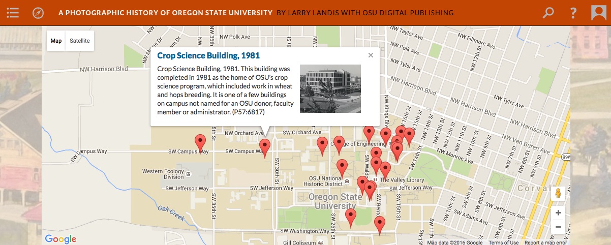Figure 1. Google Map Layout. Taken from Larry Landis’ A Photographic History of Oregon State University.

This is the second installment in a series on new layout options in Scalar 2. If you missed our prior piece on Media Gallery layouts, you can always view it here. Today we’ll be discussing the new Google Map layout.

The Google Map layout plots the current page plus any content it contains or tags on a Google Map embedded at the top of the page. Every item to be plotted must include either dcterms:coverage or dcterms:spatial metadata in the format of decimal latitude, decimal longitude. Each pin shown on the map will reveal the title, description, thumbnail and link for its content when clicked (see Figure 1). The rest of the page follows the Basic layout, with text and media interspersed.

Let’s walk through an example. I’m writing about architecture in Los Angeles. At this point my project contains several paths each of which cut through my material along a different vector. For instance, my readers can move along one path containing pages relating to individual architects; another related to design movements; and yet another containing pages related to specific architectural icons in the Los Angeles area. This third path is arranged chronologically, acting as a kind-of timeline for cutting-edge architecture in LA. But I’d also like my readers to be able to navigate those same pages discussing individual architectural structures geographically, not just chronologically. That is, I’d like my readers to be able to navigate those same pages -those same architectural icons- by way of a map.

Here’s how I’d go about doing this in Scalar.

Step one: Gather metadata. First, I’d collect the latitude and longitude, expressed in decimal degrees, for each of the architectural structures I’d like to plot on a map.

Step Two: Add metadata. Second, I’d go to each of the pages discussing individual architectural icons and add metadata to those pages. In other words, I’d (1) go to the page in my Scalar project where I discuss the LAX Theme Building; (2) click on edit to go to the edit page; (3) click on “Metadata” just below the text editor on the edit page; (4) click “Add additional metadata”; (5) within the dialogue box that pops up, tick the box under “dcterms” for either “spatial” or “coverage”; (6) click “Add fields” at the bottom-right of the dialogue box; (7) enter the latitude and longitude for LAX (in this case, 33.9425° N, -118.4081° W) into the new field that I just added under metadata called either “dcterms:spatial” or “dcterms:coverage” (depending on which field I selected); (8) save the page. I’d repeat these steps for each of the pages I’d like to plot on the map, in each case, inputting the appropriate latitude and longitude. I’d then have several pages in my Scalar project, each discussing an individual architectural structure with geospatial metadata for the location of that structure added to its respective page.

Step three: Create a page that pulls your material together. Third, I’d create a page, called, for example, “Architectural Icons in Los Angeles” and then either (1) tag that page (“Architectural Icons in Los Angeles”) to all the pages for individual architectural structures to which I just added geospatial metadata (see Figure 2) or (2) make that page (“Architectural Icons in Los Angeles”) a path and select as items in that path all the pages for individual architectural structures to which I just added geospatial metadata (see Figure 3).

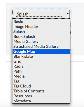
Step four: Select the Google Map layout. Finally, I would set “Architectural Icons in Los Angeles” -the page that tags or contains the other pages- to the Google Map layout. To do this, I’d click edit on “Architectural Icons in Los Angeles,” and, once in the page editor, select “Google Map” from the drop-down menu under “Layout” (see Figure 4).

In addition, the Google Map layout will also plot the current page -in our example here, the “Architectural Icons in Los Angeles” page- if it too has geospatial metadata associated with it.

But pages aren’t the type of Scalar content one can plot on a map. Once again, Scalar’s unique organizing principle in which everything is equal to everything else means that anything can do everything to anything else. In this case, it means all elements in a Scalar project can be plotted on a Google map. Or more specifically, it means that all items in a Scalar project can both have metadata associated with them and be added as a path or tagged to a page that is set to the Google Map layout. Have a set of photos taken around Los Angeles? Add geospatial metadata to those photos in Scalar and tag them to a page set to a Google Map layout. Have a video clip of twenty famous scenes all shot in Los Angeles? Annotate the video calling out those locations, add geospatial metadata to each of those annotations and then tag those annotations to a page set to the Google Map layout. Have ten short stories that each take place in a different area of Los Angeles? Make each of those stories a path in Scalar, add geospatial metadata to each of those paths (i.e. to the parent page of each path) and then tag those paths to a page set to the Google Map layout. Because tags, paths, pages, annotations, media objects and readers comments are all equivalent in Scalar, structural features -in this case, the Google Map layout- are incredibly flexible and extensible.

See you next time, when we’ll talk about the Image Header and Splash layouts.